CONTENTS

 

MUL 20

Note: GERMAN versions of the Week 20 tasks are available HERE.

 Here we look at two interpretations of division: quotition and partition (or measurement and sharing). We use a double number line (DNL) to model the two forms and try to make sense of them for different sets of numbers. Starting with a dividend of 12, we examine the models when the divisor is a factor of the dividend (3), a smaller non-whole number (2.4), a larger whole number (30) and a number less than 1 (0.3).

As we shall see, both interpretations can be made to work for all these sets of dividend-and-divisor, though in some cases neither interpretation, or only one, fits easily. It is hoped that the challenges that the students experience will deepen their understanding of division, while at the same time underlining the importance of also developing a formal understanding of division as the inverse of multiplication.

Monday: Here we use the DNL to model division as quotition (or measurement). This is straightforward and amounts to asking, 'How many 3s in 12?' and 'How many 2.4s in 12?'

You might want to take this further by asking students to think of other diagrams to represent this form of division, or to come up with stories that fit.
For example:

Toothbrushes are sold in packs of three.

How many packs are needed for 12 toothbrushes?

This diagram can also represent other operations, such as 3×4=12 and 12÷4=3.
The latter fits the partitive form of division, which we consider in Tuesday’s task:

12 toothbrushes are shared between 4 people; how many do they get each?

 

Tuesday: Here we use the DNL to model division as partition (or sharing). The resulting interpretation of 12÷3 is straightforward. For example, this simple story fits:
12 sweets are shared between 3 people; how many sweets do they get each? 

 
At first sight, such a story doesn't seem to work so well for 12÷2.4:
12 sweets are shared between 2.4 people; how many sweets do they get each?

 
However we can tweak the story to make a better fit:
12 sweets fill 2.4 packets; how many sweets fill one packet?

 
The DNL shows that the answer is 5. However, some students might reject this on the basis that the interpretation is too contrived.

Wednesday: Quentin is thinking of quotitive division again, so is asking ‘How many 30s in 12?’. This might seem a bit strange, and perhaps unanswerable for younger students, but a careful interpretation of the DNL suggests ‘about one-third’ (actually ¹²⁄₃₀ or ²⁄₅). Students might disagree as to whether this makes sense.
Parin is partitioning 12 into 30 equal parts. If this is phrased as ‘12 cakes are shared between 30 people; how many cakes do they get each?’, it may seem a bit odd, and impossible for younger students, perhaps. However, the answer of ‘about one-third’ (actually ¹²⁄₃₀ or ²⁄₅) can be read fairly readily from the DNL. This would probably make sense to more students than in Quentin’s case, especially if the matching story is rephrased slightly, with ‘how many cakes’ replaced by ‘how much cake’.

 

Thursday: Quentin is thinking of quotitive division again, so is asking ‘How many 0.3s in 12?’. This is probably easier to conceptualise than Wednesday’s ‘How many 30s in 12?’ and probably only slightly more obscure than Monday’s ‘How many 3s in 12?’, though finding the actual answer is more demanding.
Parin is partitioning 12 into 0.3 pieces, or perhaps asking 12 sweets are shared between 0.3 people; how many sweets do they get each? Neither idea seems to make immediate sense, but we could rephrase the story like this:
0.3 people get 12 sweets; how many sweets does 1 person get?
Or we could revise it like this:
12 sweets fill 0.3 packets. How many sweets fill one packet?
Students might accept that the answer of about 40, as shown on the DNL, fits one or other story well enough.

 

Friday: Here we are asking students to model quotitive and partitive division by sketching appropriate DNLs involving numbers similar to Thursday's task. Can they explain how the DNL models work?

You could again take this further by asking students to think of other diagrams to represent these two divisions, or to come up with stories that fit.

MUL 19

Note: GERMAN versions of the Week 19 tasks are available HERE.

 In this week’s tasks we focus on a family of larger and larger squares, where the multiplicative relation between the length of side of a square and that of its immediate larger neighbour is the same for all squares. The ‘super-multiplicative’ growth in the sides of the squares as we go from one square to the next, to the next, to the next.... is called exponential growth. Some of the ideas here are quite demanding, but even if they are not thoroughly understood, students can benefit from meeting this interesting (and currently, vital) mathematical concept.

Monday: Here we meet our family of exponentially growing squares. As we go from one square to the next square on the right, it soon becomes clear that the height (for example) increases by a greater amount each time. As this amount is not constant, the relation between a square’s height (h) and its family position (p) does not have a multiplicative component (m) as is found in a linear relation (a relation of the form h = mp + c). However there is a multiplicative relation between the heights of neighbouring squares. The height of A₁ is 1.2 times the height of A. The same applies to the heights of A₁ and A₂, of A₂ and A₃, etc, and so the height of A₄ is 10cm × 1.2 × 1.2 × 1.2 × 1.2 or 10cm × 1.2⁴ = 20.736cm. This is indeed about twice that of A. 

Note: Thursday’s task does involve a family of shapes where the heights increase by a constant amount, so it might help students to show it briefly here.

Some students might be happy to accept that the ×1.2 multiplicative relationship applies to all pairs of adjacent squares. However, to explain why this must be the case is not that easy. One approach is point out that the triangles above the squares are similar. An argument can be made that this means that 'sideways T-shapes', such as the red and green ones below, must be similar. Then, since the vertical limb of the red T-shape is 1.2 times the length of the horizontal limb, and equal to the horizontal limb of the next (green) T-shape, then each horizontal limb (and each vertical limb) is 1.2 times the length of its left-hand neighbour.

 

Tuesday: In this task we apply the idea that the ×1.2 relation holds between the sides of all pairs of adjacent squares. Using a calculator or spreadsheet, say, students can discover that 10×1.2¹² = 89.1610, so the sides of square A₁₂ are very close to being 9 times those of square A.

 

Wednesday: Dan would be right if the relation between square-number and side-length were linear. However, because the relation is exponential, the sides of square A₆ will √9 = 3 times those of square A rather than 9/2 = 4.5 times. Expressed formally, we can write these relations: (1.2⁶)² = 1.2¹² ≃ 9 = 3².

An empirical check of Dan and Ellie's conjectures shows that 1.2⁶ = 2.985984 ≃ 3.

 

Thursday: Here we provide a contrast to the week's previous tasks by having a family of shapes where the relationship between height and shape number is linear, rather than exponential: as can be seen, the height of adjacent rectangles increases steadily. Indeed, the height increases by 2 cm each time. Note that this time our shapes (rectangles) are not similar.

The relation between shape height (h cm) and shape number (p) can be written like this: h = 10 + 2p.

In the earlier tasks, we found that shape A₄ was roughly twice as tall as shape A. Here it happens slightly 'later': R₅ is twice as tall as R.

And previously we found that shape A₁₂ was roughly 9 times as tall as shape A. Here it happens much, much later: R₄₀ is twice as tall as R.

 

Friday: This task is challenging. It turns out that the multiplicative relation between the length of the 10mm red line and the middle red line is the same as between the middle red line and the 50mm red line.

So, if we call the multiplier m, then 10×m×m = 10m² = 50,
and so m = √5 ≃ 2.2
and so the middle red line is about 22mm long.

Students might find it hard to derive a method for finding the length of the middle red line. But nonetheless, some might hit upon the idea of multiplying 10 by the square root of 5....

We can show that 10m2 = 50, as follows.

These two triangles are similar.→

If the scale factor is m, then the longer
green line is m times the shorter one.
 

 

 

These two triangles are similar.→
As the longer green line is m times the
shorter green line, the scale factor is m.
So the longer red line is m times 10m.

MUL 18

Note: GERMAN versions of the Week 18 tasks are available HERE.

 

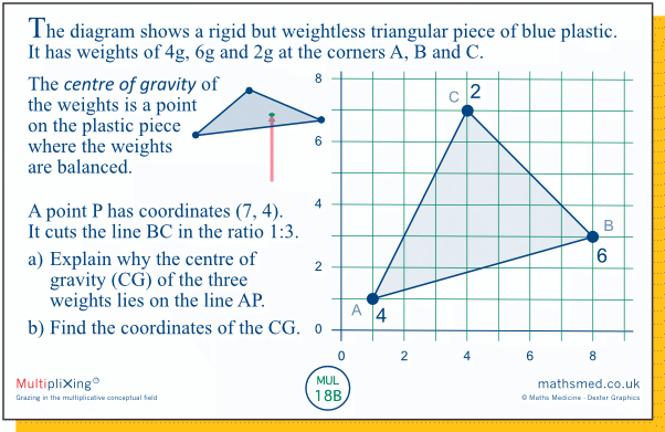
This week’s tasks involve the intriguing notion of centre of gravity (CG). This hinges on a simple relation, namely that for two weights, the ratio of their distances from the CG is the inverse of the ratio of the weights themselves. This fits with intuition, in as much as one would expect the CG to be nearer the larger weight.
However, students would benefit from knowing some physics for these tasks, especially the idea of moment of a force about a point, or more loosely for our purposes, moment of a weight about a point, which is proportional to the size of the weight and to its distance from the point. Further, and crucially, if the moments for several weights about a point ‘cancel’ out, the weights are balanced about that point and the point is the centre of gravity.
There isn’t much scope to assess or develop these notions from physics in this limited set of tasks, though a small opportunity to do so is provided in the course of Monday’s introductory task.

Monday: The main purpose of this task is to introduce the ideas needed for the rest of the week’s tasks, namely centre of gravity and the inverse relation between the ratio of a pair of weights and the ratio of the distances from their centre. As such, the task is rather perfunctory, but you might want to take the opportunity offered by the question, Can you explain why?, to explore and perhaps develop students’ knowledge of moment of a force.

The notion of moments is attractive because it is easy to apply. But for those who are unsure about why it works, it might be worth looking at another idea which seems so obvious it can be thought of as a fundamental principle:
Two identical weights are equivalent to a single weight of twice the size, operating at the point midway between them.
The principle can be applied to unequal weights too, by combining or splitting weights or parts of weights. So, for example, we can find the centre of gravity in the current task by performing the sequence of transformations below.
[Note that at each stage, the sum of the moments about P is zero.]

 Tuesday: Here we move into 2 dimensions by having three weights in a plane rather than along a rod. However, we can reduce the task to finding successive centres of gravity of pairs of weights connected by a 1 dimensional rod. Thus point P is essentially the centre of gravity of the weights from Monday's task. In turn, the centre of gravity of the three given weights is equivalent to the centre of gravity of the 4g weight at point A and an 8g weight at point P. It will thus cut the line segment AP in the ratio 8:4 or 2:1, which gives us a point with coordinates (5, 3).

The task is quite highly structured, so initially you might want to present it to students without the text, and all its hints, that comes after the second paragraph.

 

Wednesday: Here we have the same situation as in Tuesday's task, but solve it by pairing the weights in a different order. The eventual solution is of course the same.

After students have solved the task along this alternative route, you might want to suggest that they try solving it a third way, by starting with the weights at A and B. However, this is much more challenging!

Thursday: Here we start with a simple situation of four identical and symmetrically placed weights. We then modify this slightly by increasing one of the weights, which shifts the centre of gravity towards this weight.

When an extra weight is placed at point C, it will be intuitively obvious to some students that the centre of gravity shifts from P to a point closer to C. However, it might be less obvious that we can say with certainty that this new point will lie somewhere on the line segment PC.
In part b) we are told that this new point has coordinates (11, 6). This is quite near C which indicates that the extra weight is quite large....
A neat way of solving part b) is to think of the original four weights as equivalent to a weight of 4g at the point P, so that the extra weight at C becomes the only weight at C. We can then observe that the centre of gravity of the 4g weight and the extra weight at C cuts the line segment PC in the ratio 2:1. This means that these two weights are in the ratio 1:2, and so the mass of the extra weight is 8g.

 

Friday: Part a) of this task is similar to part b) of Thursday's task. A neat way to solve it is treat the configuration of the weights as equivalent to a 4g weight at the centre of the blue square and a 4g weight at C. This, in turn, is equivalent to an 8g weight at (4, 4).

 

Part b) is quite challenging in that it involves numerous steps. For example, the extra weights at A and D will have a centre of gravity on AD (obviously!) but also on y = 4 (less obviously?). So it is at (1,4). In turn this means the extra weight at D is 3 times the extra weight at A. Also, the total extra weight is half the total weight of the original weights, ie half of 8g. And so on ....

 

MUL 17

Note: GERMAN versions of the Week 17 tasks are available HERE.

 In this week's tasks we compare fractions with different denominators. Over the years, students will have met grounded methods of doing so, for example methods that involve partitioning a given shape into a carefully chosen number of equal parts. And by now they will also have met formal methods, based on transforming given fractions into equivalent fractions such that the resulting fractions have a common denominator. But even with such formal methods, it remains important that students have secure models of fractions that they can fall back on to support their thinking. So in this week's tasks we revisit the notion of fractions as parts of a whole, modelled by partitioning a shape into equal parts.

Monday: Here we use a paper strip of a certain known length as our whole. This allows us to 'quantify' the whole and to express fractions, and their difference, as quantities (specific lengths) before expressing these as fractions again. The approach is similar to Thursday's task in Week 15, where our whole was £1 and where we expressed various fractions of £1 as amounts in shillings and pence.

For an 18cm strip, it is easier to express ⅟₉ of the strip as a length than ⅛ of the strip. For the 24cm strip in part a) it is the other way round. Finding ⅟₉ of 24cm provides quite a strong test of students' basic understanding, as does the task of expressing the resulting difference, ⅓cm, as a fraction of 24cm.

 

Tuesday: Here we compare ‘adjacent’ unit fractions, starting with ⅟₈ and ⅟₉. Visually, it is difficult to ascertain their difference so we make use of a more salient comparison involving ⅟₂. In the case of ⅟₈ and ⅟₉, we first compare ⁴⁄₈ and ⁴⁄₉, where it is easy to see that ⁴⁄₈, or ⅟₂, lies exactly midway between ⁴⁄₉ and ⁵⁄₉.

In part b), the first step for Frodo's method is to compare ⁵⁄₁₀, or ⅟₂, with ⁵⁄₁₁. The difference is half of ¹⁄₁₁, or ¹⁄₂₂, so the desired difference is ¹⁄₁₁₀. Students can of course confirm this is correct by using a more formal, equivalent fractions method: ¹⁄₁₀ – ¹⁄₁₁ = ¹¹⁄₁₁₀ – ¹⁰⁄₁₁₀.
Note: This task is highly structured and it could be beneficial, and more satisfying, to loosen it. Thus, rather than simply presenting students with Frodo’s method, for them to make sense of, one could try to help them to construct the method themselves. So one could presnt students with just the diagram and then ask them to use it to find the difference between ⅟₂ and ⁴⁄₉, and then to look for a way of using the result to find the difference between ⅟₈ and ⅟₉.

 

Wednesday: Here is another way of comparing ⅛ and ⅟₉, but still using a partitioned paper strip to model the fractions. The task is quite highly structured. So initially, you might want to hide the part beneath the diagram, to give students the opportunity to think about the fraction represented by each white region without the prompts contained in that part of the task.

 

The key to Flo's method is to recognise (be it spontaneously, or through the prompts given in the task) that altogether the white regions in the given diagram cover ⅟₉ of the whole strip, because altogether the 8 tinted regions cover ⁸⁄₉ of the whole strip. The corresponding diagram for ¹⁄₁₀ – ¹⁄₁₁ would show 10 equal tinted regions, altogether covering ¹⁰⁄₁₁ of the whole strip, and 10 equal white regions altogether covering the remaining ¹⁄₁₁ of the whole strip. So one white strip, which represents ¹⁄₁₀ – ¹⁄₁₁, would cover ¹⁄₁₁₀ of the whole strip.

Thursday: Here we use a circular disc as our whole, rather than a rectangular strip. Apart from that, the method used to find the desired fraction is the same as Flo’s method in Wednesday’s task.

Students are told that each yellow region shows the difference between ⅕ and ⅙ of the disc. Can they see why?  And can they see that altogether the yellow regions cover ⅙ of the disc?

Friday: This shows a variant on Thursday's task that is slightly more general and perhaps slightly more demanding. We are told that each white region covers ⅟₇ of the circular disc. But there are only 5 such regions rather than 6, so altogether the 5 yellow regions cover two- rather than one-seventh of the disc, and so each yellow region covers ²⁄₃₅ of the disc.

It can be useful and illuminating for students to find ways to check their answer.
One approach would be formally to calculate  ⅟₅ –  ⅟₇ using the common denominator 35.

A more grounded version of this would be to express the regions in the diagram as 35ths: we have found that a yellow region represents ²⁄₃₅ of the disc; a ⅟₇ region can be written as ⁵⁄₃₅; if we add these regions, do we get ⅟₅ of the disc?

MUL 16

Note: GERMAN versions of the Week 16 tasks are available HERE.

 In this week's tasks we consider the squares of numbers, as we did in Week 2, but this time with a more sustained focus on the difference of two squares. Formally, this relation can be derived from the fact that when we expand the brackets in (a + b)(a – b), the two ab terms cancel out and we are left with a² – b². However, we take a more grounded approach in this set of tasks, in that we infer the rule from specific numerical cases, in particular cases where a – b = 1. We then suggest a way of verifying the rule (for a – b = 1) using an argument based on structural arithmetic. 

Monday: The desired value here is 32.6 + 31.6 = 64.2, using the difference of two squares. However, we don't expect students to know the relation at this point, which makes the task much more challenging.

One powerful approach is to use structural arithmetic:
32.6 × 31.6 = 31.6² plus an extra 31.6;
32.6 × 32.6 = 32.6 × 31.6 plus an extra 32.6

An equivalent approach is to use the area model: we can think of a 32.6 units square as consisting of a 31.6 units square with a 31.6 by 1 strip (blue) along one edge, and then a 32.6 by 1 strip (red) along an edge perpendicular to the first edge. 

 Tuesday: This mirrors the Week 2 Monday task. Do students have a sense that the difference between the squares of consecutive (or equally spaced) numbers increases as the numbers increase?

One approach that students might use is to consider some familiar square numbers and generalise from that. For example, the squares of the (positive) numbers 1, 2, and 3 are 1, 4, and 9, and 4 is closer to 1 than to 9. This suggests that 30² is closer to 29² than to 31².
Of course, we can’t always make a valid generalisation from a single case, though intuition suggests it must work here: how could the squares of other (positive) consecutive numbers possiby behave differently?! We can prove the result by, for example, using the area-model diagram in task 02B, or algebraically, as here:
The squares of the (positive) consecutive numbers a, a+1 and a+2 are
a², a² + 2a + 1 and a² + 4a + 4,
so the differences are 2a + 1 and 2a + 3,
and 2a + 3 > 2a + 1 (and |2a + 3| > |2a + 1| when a is positive).
Note: In the task we deliberately refer to the expressions 292, 302 and 312 as numbers, to make the point that we can think of expressions as numbers even when we haven’t found their value. You might need to clarify this for students.

 

Wednesday: Jay's equations confirm that 30² is closer to 29² than to 31² (Tuesday's task). Jay's rule can be expressed as a² – b² = a + b (for the kinds of numbers we are dealing with here, ie where a – b = 1). 

It is likely that students will be able to spot Jay's rule (though they might not express it in such a formal way). Explaining why the rule works is more challenging. One approach that students might use is to again turn to more familiar numbers and to confirm that the rule works there too. But, of course, confirming a rule is not the same as proving it. We examine a structural argument that could form the basis of a proof in Thursday's task.

 

Thursday: This is a highly structured task and it is possible that some students who manage to complete the steps will do so without much insight. You might want to probe students' understanding by asking them to execute the steps for another pair of consecutive square numbers and, more revealing perhaps, for a pair of non-consecutive square numbers (as in Friday's task).

 

Friday: Here we extend the work by considering the squares of numbers whose difference is 2 rather than 1. You might want to extend this further by considering the squares of any two (whole?) numbers.

One way to explain Elle’s rule is to use Thursday’s structural arithmetic approach. So, for 262 – 242, say, whose value can be expressed as 2(26 + 24),
we can write this:
24×26 is 24×2 or 2×24 more than 242.
26×26 is 2×26 more than 24×26.
So 262 is 2×24 + 2×26 = 2(26 + 24) more than 242.

MUL 15

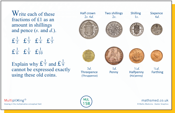
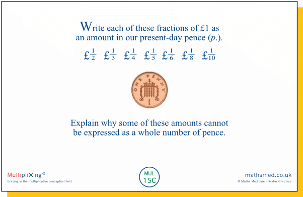
In this week's tasks we express amounts of money as fractions of £1, set in the context of the coinage that was in use in the UK before decimalisation in 1971. Decimalisation simplified the currency but we lost some of the nice numerical relations that stemmed, primarily, from the fact that there were 12 (old) pence in one shilling. There are, of course, more factors in 12 than in 10! And a lot more factors in 240 than in 100....

Monday: Here we express each of the 8 coins that were in circulation at the time, as a fraction of £1. You might want to make clear to students that 1 old pence (1d.) does not have the same value as 1 new pence (1p.)

Rather than work through the coins in the order given here (from largest denomination to smallest), you might want to encourage students to reflect on the nature of the fractional relationships by suggesting that they choose an order that they think might be easier. Having found a fraction for one coin, how easily can it be used to find a fraction for another coin?

 

Tuesday: Here we find fractional amounts of £1, using unit fractions from 1/2 to 1/10. It turns out (see Wednesday's task) that more of these amounts can expressed as a whole number of (old) pence (or other coins) than is the case with (new) pence. Why?

Rather than work through the fractional amounts in order, you might want to suggest to students that they choose an order that they think might be easier. Some student might, quite sensibly, express each amount just in pence. If so, ask them to also express the amounts in as few coins as possible. And ask whether they could have found such amounts without expressing them in pence first.

  

Wednesday: Here is a simpler, neater (?), less interesting (?) version of Tuesday's task. As students will probably have realised by now, 100 has fewer factors than 240!

Thursday: When we work with fractions, rather than thinking of them as pure numbers, we often think of them as parts of a whole (a cake, a bar of chocolate, a rectangle). It can sometimes be helpful to ‘quantify’ this whole (in terms of its price, or weight, or area, etc) and then to work with these quantities rather than with the fractions themselves, before linking the quantities back to fractions again. That is what we do here (and again in Monday’s task of Week 17).

 

We have given the answers to the three fraction additions shown in this task, to emphasise that our prime aim here is not to perform the computations but to explore (or revisit) a method that may throw light on them. After students have worked through the task, you might want to ask them what other methods could be used to check the answers.

Friday: Here we relate old pence to new pence. The fractions can be derived in a variety of ways. In the case of the first fraction, we could, for example, relate fractions to fractions (⅛ : ⅕); or we could express the numerator and denominator in terms of the same quantity (for example 30d./48d.); or we could transform the fraction into something potentially simpler (for example 5 × 2s.6d. / £1).

Some students might find these fractions quite challenging, in which case ask them to focus on just one - or nominate one for the whole class.

 

MUL 14

Note: GERMAN versions of the Week 14 tasks are available HERE.

 This week we start by revisiting some of the tasks from Week 3 but this time we examine how models (such as the double number line and Cartesian graph) can help reveal whether a relationship is multiplicative or additive.

Monday: The double number line is a very powerful representation but it can take a while for students to become familiar with it and to appreciate the significance of the fact that for a multiplicative relationship the two scales are linear and the 0s are aligned. 

The given double number line is for Paul's colour. Crucially, in this mixing-paint context, an increment of 1 unit on the white-paint scale does not match an increment of 1 unit on the black-paint scale. Specifically, while 12 is aligned with 7, we can see that 13 is not aligned with 8: for 13 tins of white paint, Vince would need slightly less than 8 tins of black paint to match Paul's colour. So Vince's colour is darker than Paul's.

Do students realise that the given double number line is for Paul's colour? Any pair of vertically aligned numbers, not just 12 and 7, gives us quantities of white and black paint that produce Paul's shade of grey.

 

Tuesday: Here we use the Cartesian plane to represent the paint mixtures. This is another powerful model, but we shouldn't assume that this power is automatically grasped by students. Using a point to represent a pair of numbers is quite a strange (and remarkable) thing to do. And while the graph produces a very tangible image, one that we can point to, talk about and embellish, we should bear in mind that it is quite abstract - it in no way resembles mixtures of tins of paint!

The line though the origin and the point (12, 7) is the set of points representing quantities of white and black paint that produce Paul's shade of grey. Points above that line, including Vince's point (13, 8) represent darker mixtures.

 

It can be useful to consider the line through the two given points (12, 7) and (13, 8). Some students might well think that the points on this line represent the same shade of grey. However, this becomes less and less plausible as we consider points nearer and nearer to the x-axis, such as (8, 3), (7, 2), (6, 1) and, perhaps, (5, 0). It seems likely that students will realise that, in some sense, white is becoming more and more 'dominant'!

 

Further, if we take the mixture represented by (6, 1), say, and combine it with the identical mixture to produce a mixture of the same colour represented by (12, 2), it is plain that this must be lighter than Paul's mixture, represented by (12, 7).

 

Wednesday: The graph shows that Salvo and José are climbing the steps at the same speed: the line joining the two given points has a slope of 1; as Salvo climbs another 20 steps, so does José. However, we should not assume that all students can read the graph in this fluent way.

We should again bear in mind that the graph is quite abstract and that some students might try to interpret it in a more concrete way: for example, they might see the lower point as representing Salvo’s position and the upper point as representing José’s at a particular time, with perhaps even an imagined zig-zag line of steps joining them.

Thursday: This task involves a geometric context, consisting of two different-sized T-shapes. Are the shapes similar? Is one an enlargement of the other? We use a 'ratio table' to represent the information, although this is perhaps a misnomer since the table per se can not tell us what kind of relationship there might be between the various dimensions. However, the table can be very useful for organising the given information so that one can more easily think about the possible relationships.

It turns out that the same additive relationship holds within each shape's horizontal and vertical limb, whereas there is no consistent multiplicative relationship. So the T-shapes are not similar. Students might notice that the green T-shape is more 'square' than the red T-shape. In a family of T-shapes with this additive relation, the taller the shape, the more square it becomes.

 

Friday: This task involves the same shapes and the same 2 by 2 table as Thursday's task. This time we look at the relation between corresponding parts of the red and green shapes. Again, we find a consistent additive rather than multiplicative relationship. So again, we can conclude that the shapes are not similar.

MUL 13

Note: GERMAN versions of the Week 13 tasks are available HERE.

 In this week's tasks we take a sideways look at fraction multiplication, using area of a rectangle as a model. A common way of introducing the model is to partition a rectangle into equal parts, and then to partition the partitions, and then finally to ask students to quantify the result. In these tasks we work the other way round, by presenting students with a carefully chosen fractional part of a rectangle in the hope that students will construct suitable partitionings for themselves.

Monday: Here we can arrive at the tinted region by halving the rectangle with a vertical cut, and then cutting one of the pieces horizontally into three equal parts. Or we could proceed the other way round: cut the rectangle into three equal horizontal strips and then halve one of the strips with a vertical cut. Either way, it is fairly obvious that six versions of the tinted piece will exactly cover the rectangle, so the tinted region covers ⅙ of the large rectangle.

 

It is possible that some students will find the desired fraction by calculating the actual areas of the two rectangles and expressing one area as a fraction of the other (ie 12×42 = 504 / 36×84 = 3024). However, a brief class discussion should soon make it clear that the task is such that there is a quicker way!

Tuesday: Here we make explicit that Monday’s tinted region can be thought of as one third of one half of the large rectangle.
Notice that in our diagram we have only cut one of the halves into thirds rather than the whole rectangle. This is a more accurate representation of ‘⅓ of ½’ than halving the rectangle and then cutting the whole rectangle into thirds, as is commonly done. However, it does not explicitly show that the resulting piece is ⅙ of the large rectangle. This might be seen as a drawback, but it has the beneficial effect of prompting students to think about the relative size of the pieces.

The two tinted regions are very differently shaped rectangles, though students may well predict that they cover the same area, as indeed they do. As with the first tinted region, the second can be thought of as ⅓ of ½ of the large rectangle or as ½ of ⅓.

 

Wednesday: Given the seemingly random position of the tinted region, students might be tempted to find the actual areas of the blue region and the whole rectangle. However, they might notice that 13 is ¼ of 52 and that 36 is ⅗ of 60, especially if they imagine the tinted region pushed to fit into one of the corners of the rectangle. So the tinted region is ⅗ of ¼ = 3/20 of the whole rectangle.

 

Some students might decide to draw a diagram, for example like the one below, to help solve the task. It can also be useful to do so after the task have been solved, especially for students who adopted a numerical approach, as this can throw light on the arithmetic.

Thursday: Here we have made things slightly more obscure - they should become clearer if one imagines the tinted region turned through 90˚.

It is fairly easy to spot that 12 is ¼ of 48, but it is probably less obvious that 45 is ³⁄₁₀ of 150. Once these fractions have been found, we can express the tinted region as ³⁄₁₀ of ¼ of the whole rectangle (or ¼ of ³⁄₁₀). How readily do students see that each of the resulting 3 pieces are 40ths of the rectangle? Again, a diagram might help, for example like the one below.
Do any students resort to decimals: 0.25 × 0.3 = 0.075? If so, can they express 0.075 as a vulgar fraction?

Friday: It is sometimes easy, and useful, to make only parallel rather than orthogonal cuts when partitioning a rectangle into a fraction of a fraction. That is the case here, where we investigate fractions of a fraction that result in one half.

In this special set of fractions of a fraction, parallel cuts work very nicely - one can see fairly clearly that the result is always one half. Interestingly, the parallel cuts also make it easier to interpret the situation as scaling, especially if we make the rectangle look more strip-like.

Parallel cuts can also be made to work in less simple cases, such as ⅕ of ⅔. Here it would not be easy, or particularly helpful, to cut the ⅔ region into just 5 equal parts using cuts parallel to the previous cuts (below, left); however, the result is perfectly easy to achieve and to read if  two ⅓ pieces are each cut into five (below right): we would then want 2 of the resulting small pieces, of which there would be 15 if the cuts were applied to the whole rectangle.